
The mutual information between two things is a measure of how much knowing one thing can tell you about the other thing. In this respect, it’s a bit like correlation, but cooler – at least in theory.
Suppose we have accumulated a lot of data about the size of apartments and their rent and we want to know if there is any relationship between the two quantities. We could do this by measuring their mutual information.
Say, for convenience, we’ve normalized our rent and size data so that the highest rent and size are 1 “unit” and the smallest ones are 0 “units”. We start out by plotting two dimensional probability distributions for the rent and size.

We plot rent on the x-axis, size on the y-axis. The density – a normalized measure of how often we run into a particular (rent,size) combination), and called the joint distribution (
So, here the joint distribution of rents and sizes (

To recall a bit of probability, and probability distributions, the probability of finding a house/apartment within a certain rent/size range combo is given by the volume of the plot within that rent/size range. The volume of the whole plot, is therefore, equal to 1, since all our data is within this range.
The mutual information is given by the equation:
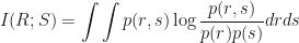
This equation takes in our rent/size data and spits out a single number. This is the value of the mutual information. The logarithm is one of the interesting parts of this equation. In practice the only effect of changing the base is to multiply your mutual information value by some number. If you use base 2 you get out an answer in ‘bits’ which makes sense in an interesting way.
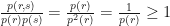
Intuitively we see that, for this data, knowing the rent tells us nothing additional about the size (and vice versa).
If we work out the value of the mutual information by substituting the values for

So we have 0 bits of information in this relation, which jives with our intuition that there is no information here – rents just don’t tell us anything about size.
Now suppose our data came out like this.

[one-bit diagram]
Substituting the values we see that (noting we have two areas to integrate, each of size 1/2 x 1/2 = 1/4)

That’s interesting. We can see intuitively there is a relation between rent and size, but what is this 1 bit of information? One way of looking at our plot is to say, if you give me a value for rent, I can tell you in which range of sizes the apartment will fall, and this range splits the total range of sizes in two. 
Interestingly, if you tell me the size of the apartment, I can tell you the range of the rent, and this range splits the total range of rents in two, so the information is still 1 bit. The mutual information is symmetric, as you may have noted from the formula.
Now, suppose our data came out like this.

[two-bit diagram]
You can see that:

Two bits! The rents and sizes seem to split into four clusters, and knowing the rent will allow us to say in which one of four clusters the size will fall. Since 
Now so far, this has been a bit ho-hum. You could imagine working out the correlation coefficient between rent and size and getting a similar notion of whether rents and sizes are related. True, we get a fancy number in bits, but so what?
Well, suppose our data came out like this.

[two-bit, scrambled diagram]
It’s funny, but the computation for MI comes out exactly the same as before:
Two bits again! There is no linear relationship that we can see between rents and sizes, but upon inspection we realize that rents and sizes cluster into four groups, and knowing the rent allows us to predict which one of four size ranges the apartment will fall in.
This, then, is the power of mutual information in exploratory data analysis. If there is some relationship between the two quantities we are testing, the mutual information will reveal this to us, without having to assume any model or pattern.
However, WHAT the relationship is, is not revealed to us, and we can not use the value of the mutual information to build any kind of predictive “box” that will allow us to predict, say, sizes from rents.
Knowing the mutual information, however, gives us an idea of how well a predictive box will do at best, regardless of whether it is a simple linear model, or a fancy statistical method like a support vector machine. Sometimes, computing the mutual information is a good, quick, first pass to check if it is worthwhile spending time training a computer to do the task at all.
A note on computing mutual information
In our toy examples above it has been pretty easy to compute mutual information because the forms of 
You will notice that the term in the integral is always positive. 


You will immediately sense the problem here. In many calculations, when we have noise in the terms, the noise averages out because the plus terms balance out the minus terms. Here, all we have are plus terms, and our integral has a tendency to get bigger.

Histograms (where we take the data and bin it) is an expedient way of estimating probability distributions and they normally work alright. But this can lead us to a funny problem when computing mutual information because of this always positive nature of the integral term.
For example, say there was really no dependence between rents and sizes, but suppose our data and our binning interacted in an odd manner to give us a pattern such as this:

[checkerboard]
We can see that the marginals are not affected badly, but the joint, because it is in two-dimensional space, is filled rather more sparsely which leads to us having ‘holes’ in the distribution. If we now compute the mutual information we find that we have ended up with 1 bit of information, when really, it should be 0 bits.
Most attempts to address this bias in mutual information computations recognize the problem with these ‘holes’ in the joint distribution and try to smear them out using various ever more sophisticated techniques. The simplest way is to make larger bins (which would completely solve our problem in this toy case) and other methods blur out the original data points themselves.
All of these methods, not matter how fancy, still leave us with the problem of how much to smear the data: smear too little and you inflate the mutual information, smear too much and you start to wipe it out.
Often, to be extra cautious, we do what I have known as ‘shuffle correction’ (and I was told by a pro is actually called the ‘null model’). Here you thoroughly jumble up your data so that any relation ship that existed between r and s is gone. You then compute the mutual information of that jumbled up data. You know that the mutual information should actually be zero, but because of the bias it comes out to something greater. You then compare the mutual information from the data with this jumbled one to see if there is something peeking above the bias.

Oh, also: http://www.youtube.com/watch?v=iUrzicaiRLU
A VERY nice set of examples! Thanks!
Hey thanks!